Export Pixie data in the OpenTelemetry format.Learn more🚀
Pixie has an OpenTelemetry plugin!
Ctrl/Cmd + K
Building a Continuous Profiler Part 2: A Simple eBPF-Based Profiler


Omid Azizi, Pete Stevenson
June 01, 2021 • 5 minutes readPrincipal Engineer @ New Relic, Founding Engineer @ Pixie Labs
Principal Engineer @ New Relic, Founding Engineer @ Pixie Labs
In the last blog post, we discussed the basics of CPU profilers for compiled languages like Go, C++ and Rust. We ended by saying we wanted a sampling-based profiler that met these two requirements:
Does not require recompilation or redeployment: This is critical to Pixie’s auto-telemetry approach to observability. You shouldn’t have to instrument or even re-run your application to get observability.
Has very low overheads: This is required for a continuous (always-on) profiler, which was desirable for making performance profiling as low-effort as possible.
A few existing profilers met these requirements, including the Linux perf tool. In the end, we settled on the BCC eBPF-based profiler developed by Brendan Gregg [1] as the best reference. With eBPF already at the heart of the Pixie platform, it was a natural fit, and the efficiency of eBPF is undeniable.
If you’re familiar with eBPF, it’s worth checking out the source code of the BCC implementation. For this blog, we’ve prepared our own simplified version that we’ll examine in more detail.
An eBPF-based profiler
The code to our simple eBPF-based profiler can be found here, with further instructions included at the end of this blog (see Running the Demo Profiler). We’ll be explaining how it works, so now’s a good time to clone the repo.
Also, before diving into the code, we should mention that the Linux developers have already put in dedicated hooks for collecting stack traces in the kernel. These are the main APIs we use to collect stack traces (and this is how the official BCC profiler works well). We won’t, however, go into Linux’s implementation of these APIs, as that’s beyond the scope of this blog.
With that said, let’s look at some BCC eBPF code. Our basic structure has three main components:
const int kNumMapEntries = 65536;BPF_STACK_TRACE(stack_traces, kNumMapEntries);BPF_HASH(histogram, struct stack_trace_key_t, uint64_t, kNumMapEntries);int sample_stack_trace(struct bpf_perf_event_data* ctx) {// Collect stack traces// ...}

Here we define:
A
BPF_STACK_TRACEdata structure calledstack_tracesto hold sampled stack traces. Each entry is a list of addresses representing a stack trace. The stack trace is accessed via an assigned stack trace ID.A
BPF_HASHdata structure calledhistogramwhich is a map from the sampled location in the code to the number of times we sampled that location.A function
sample_stack_tracethat will be periodically triggered. The purpose of this eBPF function is to grab the current stack trace whenever it is called, and to populate/update thestack_tracesandhistogramdata structures appropriately.
The diagram below shows an example organization of the two data structures.
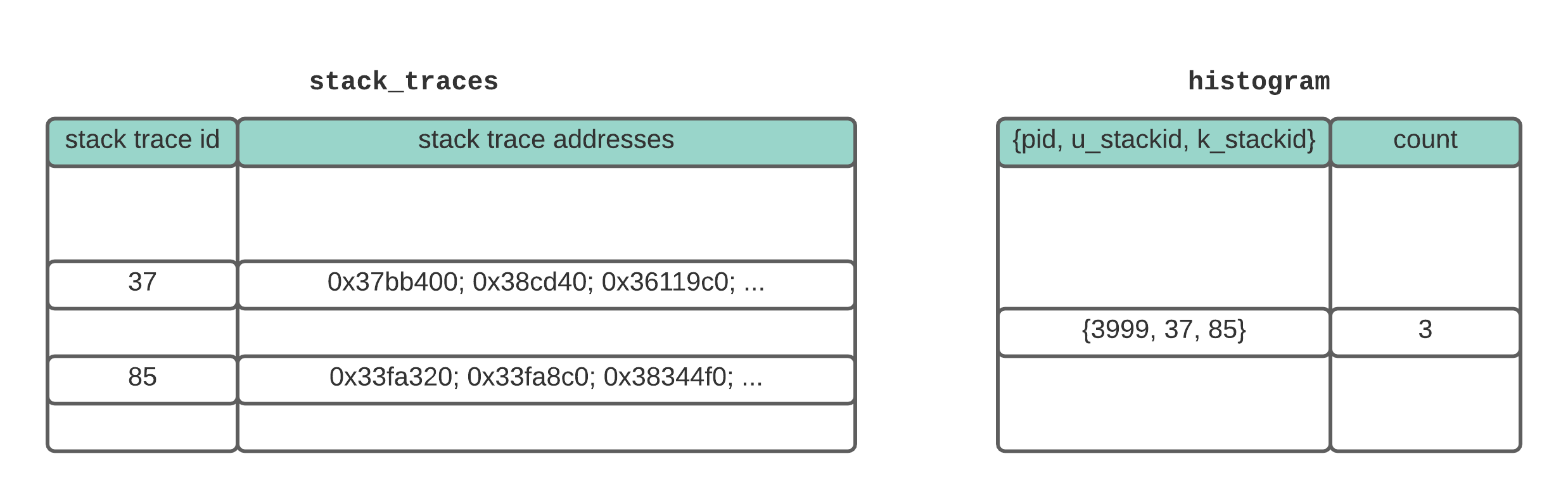
The two main data structures for our eBPF performance profiler. The stack_traces map records stack traces and assigns them an id. The histogram map counts the number of times a particular location in the code (defined by the combination of the user stack trace and kernel stack trace) is sampled.
As we’ll see in more detail later, we’ll set up our BPF code to trigger on a periodic timer. This means every X milliseconds, we’ll interrupt the CPU and trigger the eBPF probe to sample the stack traces. Note that this happens regardless of which process is on the CPU, and so the eBPF profiler is actually a system-wide profiler. We can later filter the results to include only the stack traces that belong to our application.
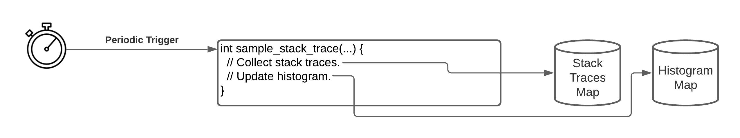
The sample_stack_trace function is set-up to trigger periodically. Each time it triggers, it collects the stack trace and updates the two maps.
Now let’s look at the full BPF code inside sample_stack_trace:
int sample_stack_trace(struct bpf_perf_event_data* ctx) {// Sample the user stack trace, and record in the stack_traces structure.int user_stack_id = stack_traces.get_stackid(&ctx->regs, BPF_F_USER_STACK);// Sample the kernel stack trace, and record in the stack_traces structure.int kernel_stack_id = stack_traces.get_stackid(&ctx->regs, 0);// Update the counters for this user+kernel stack trace pair.struct stack_trace_key_t key = {};key.pid = bpf_get_current_pid_tgid() >> 32;key.user_stack_id = user_stack_id;key.kernel_stack_id = kernel_stack_id;histogram.increment(key);return 0;}
Surprisingly, that’s it! That’s the entirety of our BPF code for our profiler. Let’s break it down...
Remember that an eBPF probe runs in the context when it was triggered, so when this probe gets triggered it has the context of whatever program was running on the CPU. Then it essentially makes two calls to stack_traces.get_stackid(): one to get the current user-code stack trace, and another to get the kernel stack trace. If the code was not in kernel space when interrupted, the second call simply returns EEXIST, and there is no stack trace. You can see that all the heavy-lifting is really done by the Linux kernel.
Next, we want to update the counts for how many times we’ve been at this exact spot in the code. For this, we simply increment the counter for the entry in our histogram associated with the tuple {pid, user_stack_id, kernel_stack_id}. Note that we throw the PID into the histogram key as well, since that will later help us know which process the stack trace belongs to.
We’re Not Done Yet
While the eBPF code above samples the stack traces we want, we still have a little more work to do. The remaining tasks involve:
Setting up the trigger condition for our BPF program, so it runs periodically.
Extracting the collecting data from BPF maps.
Converting the addresses in the stack traces into human readable symbols.
Fortunately, all this work can be done in user-space. No more eBPF required.
Setting up our BPF program to run periodically turns out to be fairly easy. Again, credit goes to the BCC and eBPF developers. The crux of this setup is the following:
bcc->attach_perf_event(PERF_TYPE_SOFTWARE,PERF_COUNT_SW_CPU_CLOCK,std::string(probe_fn),sampling_period_millis * kNanosPerMilli,0);
Here we’re telling the BCC to set up a trigger based on the CPU clock by setting up an event based on PERF_TYPE_SOFTWARE/PERF_COUNT_SW_CPU_CLOCK. Every time this value reaches a multiple of sampling_period_millis, the BPF probe will trigger and call the specified probe_fn, which happens to be our sample_stack_trace BPF program. In our demo code, we’ve set the sampling period to be every 10 milliseconds, which will collect 100 samples/second. That’s enough to provide insight over a minute or so, but also happens infrequently enough so it doesn’t add noticeable overheads.
After deploying our BPF code, we have to collect the results from the BPF maps. We access the maps from user-space using the BCC APIs:
ebpf::BPFStackTable stack_traces =bcc->get_stack_table(kStackTracesMapName);ebpf::BPFHashTable<stack_trace_key_t, uint64_t> histogram =bcc->get_hash_table<stack_trace_key_t, uint64_t>(kHistogramMapName);
Finally, we want to convert our addresses to symbols, and to concatenate our user and kernel stack traces. Fortunately, BCC has once again made our life easy on this one. In particular, there is a call stack_traces.get_stack_symbol, that will convert the list of addresses in a stack trace into a list of symbols. This function needs the PID, because it will lookup the debug symbols in the process’s object file to perform the translation.
std::map<std::string, int> result;for (const auto& [key, count] : histogram.get_table_offline()) {if (key.pid != target_pid) {continue;}std::string stack_trace_str;if (key.user_stack_id >= 0) {std::vector<std::string> user_stack_symbols =stack_traces.get_stack_symbol(key.user_stack_id, key.pid);for (const auto& sym : user_stack_symbols) {stack_trace_str += sym;stack_trace_str += ";";}}if (key.kernel_stack_id >= 0) {std::vector<std::string> user_stack_symbols =stack_traces.get_stack_symbol(key.kernel_stack_id, -1);for (const auto& sym : user_stack_symbols) {stack_trace_str += sym;stack_trace_str += ";";}}result[stack_trace_str] += 1;}
It actually turns out that the process of turning the stack traces into symbols is the part of this process that introduces the most overhead. The actual sampling of stack traces is negligible. Our next blog post will discuss the performance challenges of making this basic profiler ready for production.
Running the Demo Profiler
Running the simple CPU profiler.
The code and instructions for running the simple eBPF based profiler can be found here.
The code was designed to have as few dependencies as possible, but you need BCC installed. Follow the instructions in README.md for more details on building the profiler and a toy app to profiler.
Once built, you can run the profiler as follows:
# Profile the application for 30 seconds.sudo ./perf_profiler <target PID> 30
You should see stack traces from the target program like the following:
Successfully deployed BPF profiler.Collecting stack trace samples for 30 seconds.1 indexbytebody;runtime.funcname;runtime.isAsyncSafePoint; … ;runtime.goexit;5 main.main;runtime.main;runtime.goexit;24 main.sqrt;runtime.main;runtime.goexit;
You can then experiment by running it against other running processes in your system. Some processes may not have debug symbols installed, in which case you will see the [UNKNOWN] marker.
Another fun experiment is to run it against a program written in a different language, like Python or Java. You’ll see stack traces, but they’re probably not what you’re expecting. For example, with Python, what you’ll see is the Python interpreter’s stack traces rather than the Python application (Note: you’ll need the interpreter’s debug symbols to see the functions; On Ubuntu, you can get these by running something like apt install python3.6-dbg) . We’ll cover profiling for Java and interpreted languages in a future post.
In part three of this series, we’ll discuss the challenges we faced in building out this simple profiler into a production ready profiler.
Related posts


Terms of Service|Privacy Policy
We are a Cloud Native Computing Foundation sandbox project.

Pixie was originally created and contributed by New Relic, Inc.
Copyright © 2018 - The Pixie Authors. All Rights Reserved. | Content distributed under CC BY 4.0.
The Linux Foundation has registered trademarks and uses trademarks. For a list of trademarks of The Linux Foundation, please see our Trademark Usage Page.
Pixie was originally created and contributed by New Relic, Inc.
This site uses cookies to provide you with a better user experience. By using Pixie, you consent to our use of cookies.