Export Pixie data in the OpenTelemetry format.Learn more🚀
Pixie has an OpenTelemetry plugin!
Ctrl/Cmd + K
Building a Continuous Profiler Part 3: Optimizing for Prod Systems


Pete Stevenson, Omid Azizi
August 16, 2021 • 5 minutes readPrincipal Engineer @ New Relic, Founding Engineer @ Pixie Labs
Principal Engineer @ New Relic, Founding Engineer @ Pixie Labs
This is the third part in a series of posts describing how we built a continuous (always-on) profiler for identifying application performance issues in production Kubernetes clusters.
We were motivated to build a continuous profiler based on our own experience debugging performance issues. Manually profiling an application on a Kubernetes node without recompiling or redeploying the target application is not easy: one has to connect to the node, collect the stack traces with an appropriate system profiler, transfer the data back and post-process the results into a useful visualization, all of which can be quite frustrating when trying to figure out a performance issue. We wanted a system-wide profiler that we could leave running all the time, and which we could instantly query to get CPU flamegraphs without any hassle.
In Part 1 and Part 2, we discussed the basics of profiling and walked through a simple but fully functional eBPF-based CPU profiler (inspired by the BCC profiler) which would allow us to capture stack traces without requiring recompilation or redeployment of profiled applications.
In this post, we discuss the process of turning the basic profiler into one with only 0.3% CPU overhead, making it suitable for continuous profiling of all applications in production systems.
Profiling the profiler
To turn the basic profiler implementation from Part 2 into a continuous profiler, it was just a “simple” matter of leaving the eBPF profiler running all the time, such that it continuously collects stack traces into eBPF maps. We then periodically gather the stack traces and store them to generate flamegraphs when needed.
While this approach works, we had expected our profiler to have <0.1% CPU overhead based on the low cost of gathering stack trace data (measured at ~3500 CPU instructions per stack trace)1. The actual overhead of the initial implementation, however, was 1.3% CPU utilization -- over 10x what we had expected. It turned out that the stack trace processing costs, which we had not accounted for, matter quite a lot for continuous profilers.
Most basic profilers can be described as “single shot” in that they first collect raw stack traces for a period of time, and then process the stack traces after all the data is collected. With “single shot” profilers, the one-time post-processing costs of moving data from the kernel to user space and looking up address symbols are usually ignored. For a continuous profiler, however, these costs are also running continuously and become as important as the other overheads.
With CPU overhead much higher than anticipated, we used our profiler to identify its own hotspots. By examining the flamegraphs, we realized that two post-processing steps were dominating CPU usage: (1) symbolizing the addresses in the stack trace, and (2) moving data from kernel to user space.
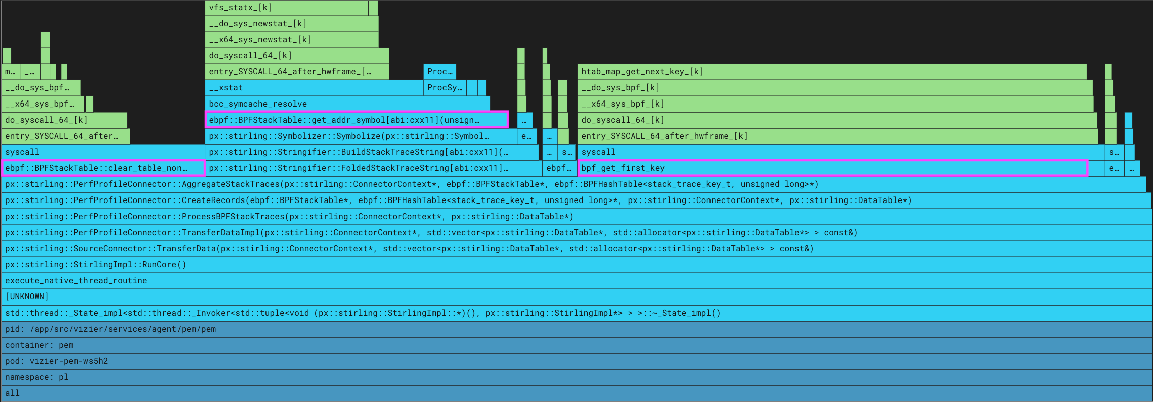
A flamegraph of the continuous profiler showing significant time spent in BPF system calls: clear_table_non_atomic(), get_addr_symbol(), bpf_get_first_key().
Performance optimizations
Based on the performance insights above, we implemented three specific optimizations:
- Adding a symbol cache.
- Reducing the number of BPF system calls.
- Using a perf buffer instead of BPF hash map for exporting histogram data.
Adding a symbol cache
For a stack trace to be human readable, the raw instruction addresses need to be translated into function names or symbols. To symbolize a particular address, ELF debug information from the underlying binary is searched for the address range that includes the instruction address2.
The flamegraph clearly showed that we were spending a lot of time in symbolization, as evidenced by the time spent in ebpf::BPFStackTable::get_addr_symbol(). To reduce this cost, we implemented a symbol cache that is checked before accessing the ELF information.
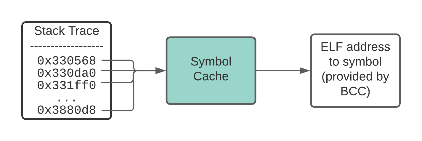
Caching the symbols for individual instruction addresses speeds up the process of symbolization.
We chose to cache individual stack trace addresses, rather than entire stack frames. This is effective because while many stack traces diverge at their tip, they often share common ancestry towards their base. For example, main is a common symbol at the base of many stack traces.
Adding a symbol cache provided a 25% reduction (from 1.27% to 0.95%) in CPU utilization.
Reducing the number of BPF system calls
From Part 2, you may recall that our profiler has two main data structures:
- A
BPFStackTablerecords stack traces and assigns them an id. - A
BPFHashTablecounts the number of times a particular location in the code (defined by the combination of the user stack trace and kernel stack trace) is sampled.
To transfer and clear the data in these structures from kernel to user space, the initial profiler implementation used the following BCC APIs:
BPFStackTable::get_stack_symbol() // Read & symbolize one stack traceBPFStackTable::clear_table_non_atomic() // Prepare for next useBPFHashTable::get_table_offline() // Read stack trace histogramBPFHashTable::clear_table_non_atomic() // Prepare for next use

Flamegraph analysis of our profiler in production showed a significant amount of time spent in these calls. Examining the call stack above get_table_offline() and clear_table_non_atomic() revealed that each call repeatedly invoked two eBPF system calls to traverse the BPF map: one syscall to find the next entry and another syscall to read or clear it.
For the BPFStackTable, the clear_table_non_atomic() method is even less efficient because it visits and attempts to clear every possible entry rather than only those that were populated.
To reduce the duplicated system calls, we edited the BCC API to combine the tasks of reading and clearing the eBPF shared maps into one pass that we refer to as “consuming” the maps.
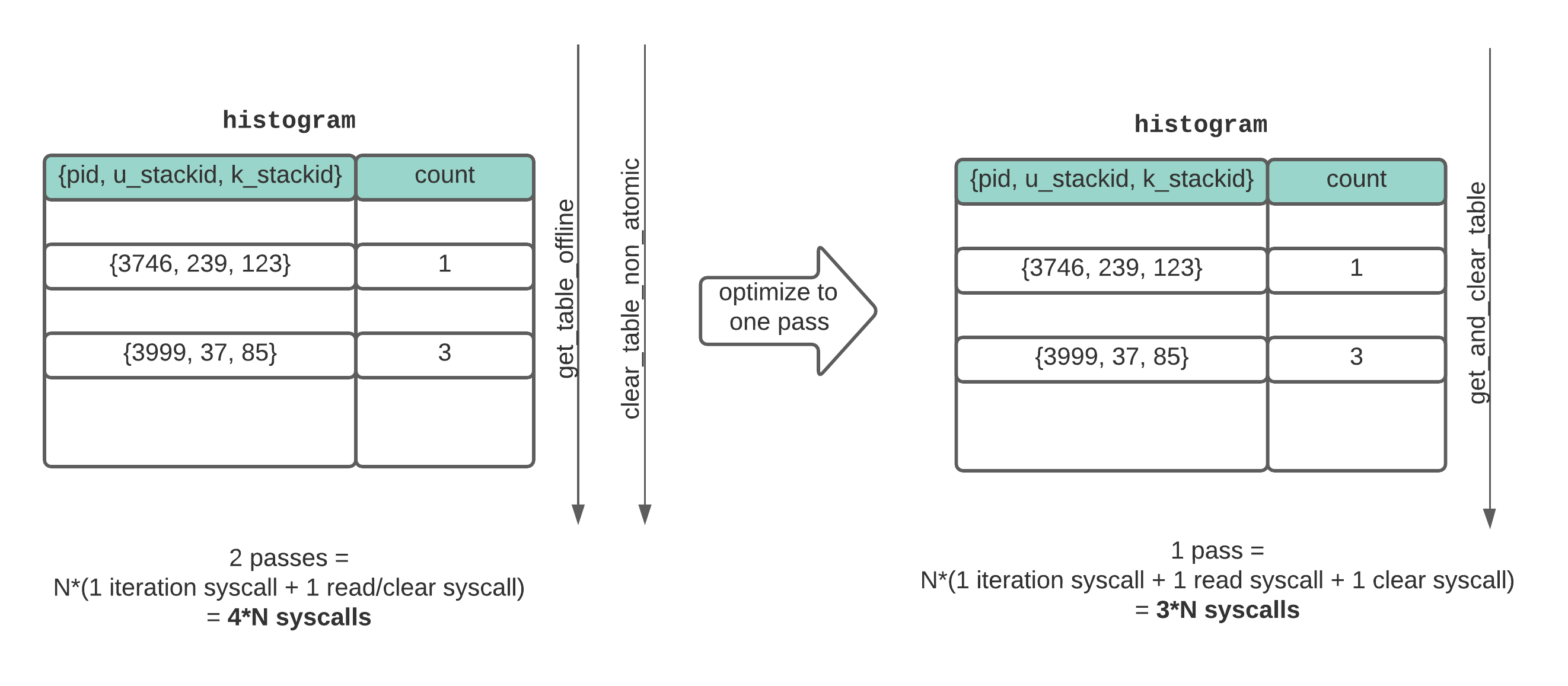
Combining the BCC APIs for accessing and clearing BPF table data reduces the number of expensive system calls.
When applied to both data structures, this optimization provided a further 58% reduction (from 0.95% to 0.40%) in CPU utilization. This optimization shows the high cost of making repeated system calls to interact with BPF maps, a lesson we have now taken to heart.
Switching from BPF hash map to perf buffer
The high costs of accessing the BPF maps repeatedly made us wonder if there was a more efficient way to transfer the stack trace data to user space.
We realized that by switching the histogram table to a BPF perf buffer (which is essentially a circular buffer), we could avoid the need to clear the stack trace keys from the map 3. Perf buffers also allow faster data transfer because they use fewer system calls per readout.
On the flip side, the BPF maps were performing some amount of stack trace aggregation in kernel space. Since perf buffers report every stack trace without aggregation, this would require us to transfer about twice as much data according to our experiments.
In the end, it turned out the benefit of the perf buffer’s more efficient transfers (~125x that of hash maps) outweighed the greater volume of data (~2x) we needed to transfer. This optimization further reduced the overhead to about 0.3% CPU utilization.
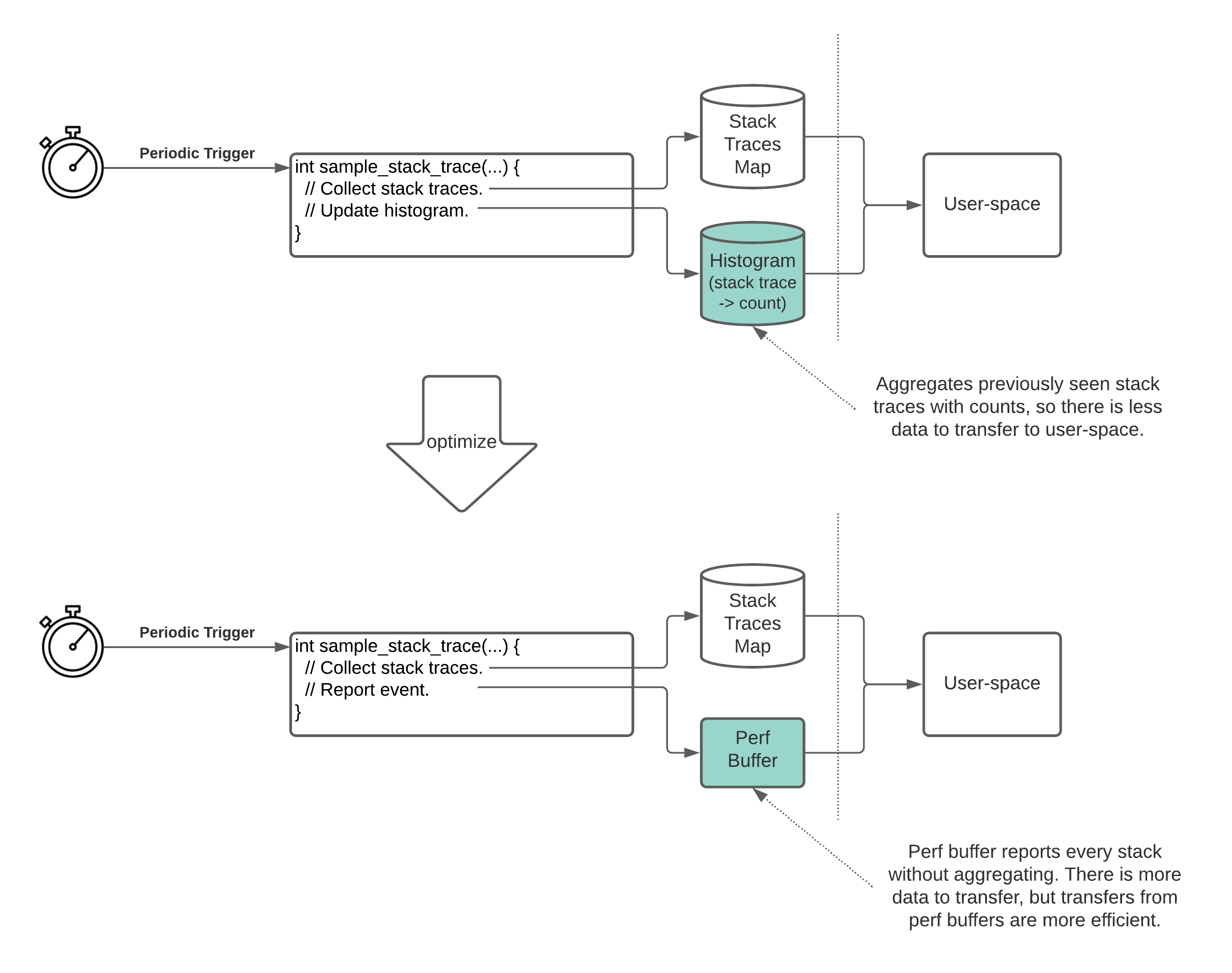
Switching a BPF hash map to a BPF perf buffer eliminates the need to clear data and increases the speed of data transfer.
Conclusion
In the process of building a continuous profiler, we learned that the cost of symbolizing and moving stack trace data was far more expensive than the underlying cost of collecting the raw stack trace data.
Our efforts to optimize these costs led to a 4x reduction (from 1.27% to 0.31%) in CPU overhead -- a level we’re pretty happy with, even if we’re not done optimizing yet.
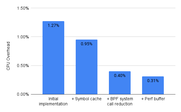
Graph of the incremental improvement in CPU utilization for each optimization.
The result of all this work is a low overhead continuous profiler that is always running in the Pixie platform. To see this profiler in action, check out the tutorial!
Footnotes
Footnotes
- Based on the following assumptions: (1) about 3500 CPU instructions executed to collect a stack trace sample, (2) a CPU that processes 1B instructions per second, and (3) a sampling frequency of 100 Hz (or 10 ms.). The expected overhead with theses assumptions is 3500 * 100 / 1B = 0.035%. Note that this figure ignores the stack trace post-processing overheads.↩
- If the ELF debug information is not available, Pixie’s profiler cannot symbolize.↩
- The Stack Traces Map cannot be converted to a perf buffer because it is populated by a BPF helper function.↩
Related posts


Terms of Service|Privacy Policy
We are a Cloud Native Computing Foundation sandbox project.

Pixie was originally created and contributed by New Relic, Inc.
Copyright © 2018 - The Pixie Authors. All Rights Reserved. | Content distributed under CC BY 4.0.
The Linux Foundation has registered trademarks and uses trademarks. For a list of trademarks of The Linux Foundation, please see our Trademark Usage Page.
Pixie was originally created and contributed by New Relic, Inc.
This site uses cookies to provide you with a better user experience. By using Pixie, you consent to our use of cookies.